A Measurement System Can Be Modeled by the Equation .5y+y=f(T)

An Introduction to the Finite Element Method

The description of the laws of physics for infinite- and time-dependent problems are usually expressed in terms of fractional differential equations (PDEs). For the vast bulk of geometries and bug, these PDEs cannot exist solved with analytical methods. Instead, an approximation of the equations can be constructed, typically based upon different types of discretizations. These discretization methods guess the PDEs with numerical model equations, which can be solved using numerical methods. The solution to the numerical model equations are, in plough, an approximation of the existent solution to the PDEs. The finite element method (FEM) is used to compute such approximations.

Have, for example, a function u that may be the dependent variable in a PDE (i.eastward., temperature, electric potential, force per unit area, etc.) The function u can be approximated by a function u_h using linear combinations of basis functions according to the following expressions:

⁽¹⁾

and

⁽²⁾

Here, ψ_i denotes the basis functions and u_i denotes the coefficients of the functions that judge u with u_h . The effigy below illustrates this principle for a 1D problem. u could, for instance, represent the temperature along the length (x) of a rod that is nonuniformly heated. Here, the linear basis functions have a value of 1 at their respective nodes and 0 at other nodes. In this case, there are 7 elements along the portion of the 10-centrality, where the function u is divers (i.e., the length of the rod).

The part u (solid blue line) is approximated with u_h (dashed red line), which is a linear combination of linear basis functions (ψ_i is represented by the solid black lines). The coefficients are denoted by u₀ through u₇ .

The function u (solid blueish line) is approximated with u_h (dashed carmine line), which is a linear combination of linear basis functions (ψ_i is represented by the solid black lines). The coefficients are denoted by u₀ through u_vii .

I of the benefits of using the finite element method is that it offers great freedom in the pick of discretization, both in the elements that may exist used to discretize space and the ground functions. In the figure above, for example, the elements are uniformly distributed over the x-axis, although this does not take to exist the case. Smaller elements in a region where the slope of u is large could also have been applied, as highlighted below.

The function u (solid blue line) is approximated with u_h (dashed red line), which is a linear combination of linear basis functions (ψ_i is represented by the solid blackness lines). The coefficients are denoted by u₀ through u₇ .

The function u (solid blueish line) is approximated with u_h (dashed red line), which is a linear combination of linear basis functions (ψ_i is represented past the solid black lines). The coefficients are denoted by u₀ through u₇ .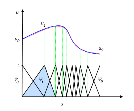

Both of these figures evidence that the selected linear basis functions include very limited support (nonzero simply over a narrow interval) and overlap along the x-centrality. Depending on the problem at hand, other functions may be chosen instead of linear functions.

Another benefit of the finite element method is that the theory is well developed. The reason for this is the close relationship between the numerical formulation and the weak formulation of the PDE problem (run into the department below). For instance, the theory provides useful fault estimates, or bounds for the error, when the numerical model equations are solved on a computer.

Looking dorsum at the history of FEM, the usefulness of the method was first recognized at the start of the 1940s by Richard Courant, a German language-American mathematician. While Courant recognized its application to a range of bug, it took several decades before the approach was applied generally in fields outside of structural mechanics, becoming what it is today.

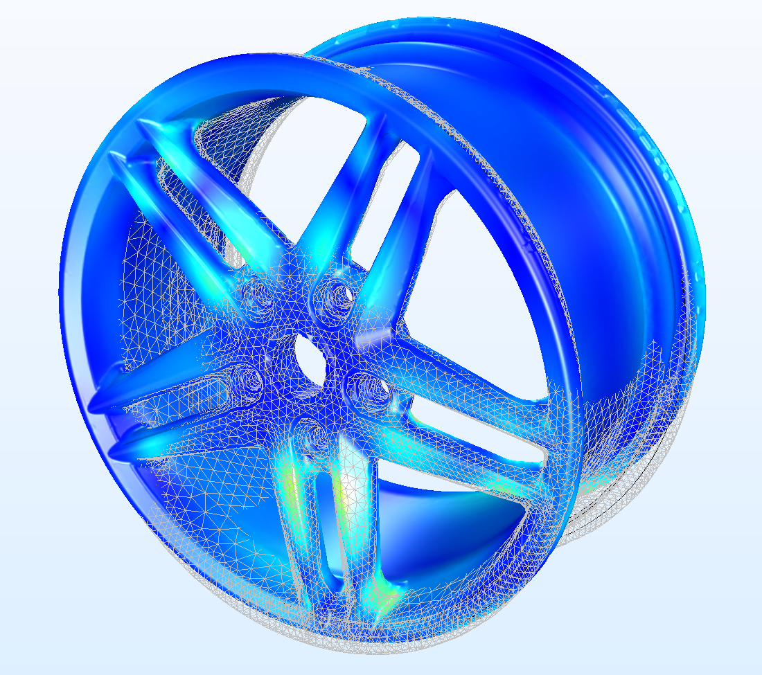Finite element discretization, stresses, and deformations of a wheel rim in a structural analysis. Finite element discretization, stresses, and deformations of a bicycle rim in a structural analysis.

Algebraic Equations, Ordinary Differential Equations, Partial Differential Equations, and the Laws of Physics

The laws of physics are often expressed in the linguistic communication of mathematics. For example, conservation laws such as the police of conservation of energy, conservation of mass, and conservation of momentum tin can all exist expressed as partial differential equations (PDEs). Constitutive relations may also be used to express these laws in terms of variables like temperature, density, velocity, electrical potential, and other dependent variables.

Differential equations include expressions that determine a minor modify in a dependent variable with respect to a change in an independent variable (ten, y, z, t). This small change is as well referred to every bit the derivative of the dependent variable with respect to the contained variable.

Say there is a solid with time-varying temperature but negligible variations in space. In this instance, the equation for conservation of internal (thermal) energy may result in an equation for the alter of temperature, with a very small change in time, due to a estrus source g:

⁽³⁾

Here, denotes the density and C_p denotes the oestrus capacity. Temperature, T, is the dependent variable and time, t, is the contained variable. The part may describe a estrus source that varies with temperature and time. Eq. (3) states that if there is a change in temperature in time, so this has to be balanced (or caused) past the oestrus source . The equation is a differential equation expressed in terms of the derivatives of one independent variable (t). Such differential equations are known as ordinary differential equations (ODEs).

In some situations, knowing the temperature at a time t₀ , called an initial condition, allows for an analytical solution of Eq. (three) that is expressed equally:

⁽⁴⁾

The temperature in the solid is therefore expressed through an algebraic equation (4), where giving a value of time, t₁ , returns the value of the temperature, T _i, at that fourth dimension.

Oftentimes, there are variations in fourth dimension and space. The temperature in the solid at the positions closer to a estrus source may, for case, be slightly higher than elsewhere. Such variations farther give rise to a oestrus flux between the different parts within the solid. In such cases, the conservation of energy tin can upshot in a heat transfer equation that expresses the changes in both fourth dimension and spatial variables (x), such as:

⁽⁵⁾

As earlier, T is the dependent variable, while ten (x = (x, y, z)) and t are the independent variables. The oestrus flux vector in the solid is denoted by q = (q_x, q_y, q_z ) while the difference of q describes the modify in heat flux along the spatial coordinates. For a Cartesian coordinate organization, the departure of q is defined equally:

⁽⁶⁾

Eq. (5) thus states that if there is a alter in internet flux when changes are added in all directions and so that the divergence (sum of the changes) of q is not nix, then this has to exist balanced (or caused) by a rut source and/or a change in temperature in time (accumulation of thermal energy).

The heat flux in a solid can be described by the constitutive relation for heat flux by conduction, likewise referred to as Fourier's law:

⁽⁷⁾

In the above equation, k denotes the thermal electrical conductivity. Eq. (seven) states that the heat flux is proportional to the gradient in temperature, with the thermal electrical conductivity as proportionality constant. Eq. (vii) in (5) gives the following differential equation:

⁽⁸⁾

Hither, the derivatives are expressed in terms of t, x, y, and z. When a differential equation is expressed in terms of the derivatives of more than ane independent variable, it is referred to every bit a partial differential equation (PDE), since each derivative may represent a alter in one direction out of several possible directions. Farther notation that the derivatives in ODEs are expressed using d, while fractional derivatives are expressed using the more curly ∂.

In addition to Eq. (viii), the temperature at a time t ₀ and temperature or heat flux at some position ten ₀ could exist known as well. Such knowledge can be applied in the initial condition and purlieus conditions for Eq. (8). In many situations, PDEs cannot be resolved with analytical methods to give the value of the dependent variables at different times and positions. Information technology may, for example, be very hard or impossible to obtain an analytic expression such as:

⁽⁹⁾

from Eq. (eight).

Rather than solving PDEs analytically, an culling option is to search for approximate numerical solutions to solve the numerical model equations. The finite element method is exactly this blazon of method – a numerical method for the solution of PDEs.

Similar to the thermal energy conservation referenced higher up, it is possible to derive the equations for the conservation of momentum and mass that form the basis for fluid dynamics. Farther, the equations for electromagnetic fields and fluxes can be derived for space- and time-dependent issues, forming systems of PDEs.

Continuing this discussion, permit'south encounter how the so-called weak formulation can be derived from the PDEs.

The Finite Element Method from the Weak Formulation: Footing Functions and Test Functions

Assume that the temperature distribution in a estrus sink is being studied, given by Eq. (viii), but now at steady state, meaning that the time derivative of the temperature field is aught in Eq. (8). The domain equation for the model domain, Ω, is the following:

^(x)

Farther, assume that the temperature along a boundary (∂Ω_i) is known, in improver to the expression for the estrus flux normal to some other boundaries (∂Ω₂). On the remaining boundaries, the heat flux is zero in the outward direction (∂Ω₃). The boundary conditions at these boundaries then become:

^(xi)

⁽¹²⁾

⁽¹³⁾

where h denotes the heat transfer coefficient and T _amb denotes the ambient temperature. The outward unit normal vector to the boundary surface is denoted past n. Equations (x) to (13) describe the mathematical model for the estrus sink, as shown below.

The domain equation and boundary conditions for a mathematical model of a estrus sink.

The domain equation and purlieus conditions for a mathematical model of a heat sink.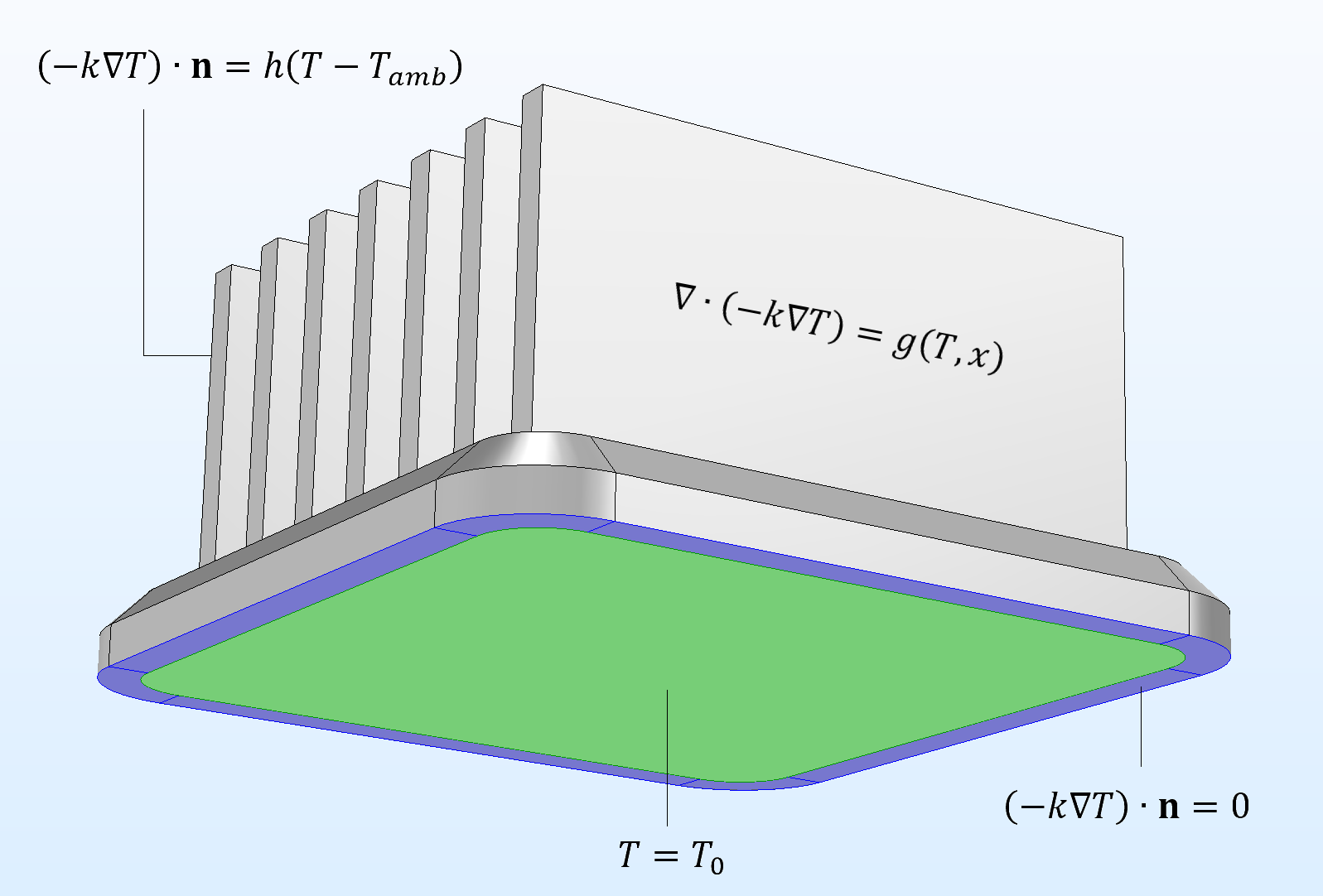

The side by side footstep is to multiply both sides of Eq. (x) past a test function φ and integrate over the domain Ω:

⁽¹⁴⁾

The test part φ and the solution T are assumed to belong to Hilbert spaces. A Hilbert space is an infinite-dimensional function infinite with functions of specific backdrop. It tin be viewed as a collection of functions with certain overnice properties, such that these functions can be conveniently manipulated in the same way as ordinary vectors in a vector infinite. For example, yous can grade linear combinations of functions in this drove (the functions have a well-defined length referred to as norm) and y'all can measure the angle between the functions, only like Euclidean vectors.

Indeed, after applying the finite element method on these functions, they are but converted to ordinary vectors. The finite element method is a systematic way to convert the functions in an infinite dimensional office space to get-go functions in a finite dimensional function space and then finally ordinary vectors (in a vector space) that are tractable with numerical methods.

The weak formulation is obtained by requiring (xiv) to concord for all examination functions in the test function space instead of Eq. (10) for all points in Ω. A trouble conception based on Eq. (ten) is thus sometimes referred to as the pointwise formulation. In the so-called Galerkin method, it is causeless that the solution T belongs to the same Hilbert space as the test functions. This is usually written equally φ ϵ H and T ϵ H, where H denotes the Hilbert space. Using Dark-green'southward beginning identity (substantially integration by parts), the post-obit equation can be derived from (14):

⁽¹⁵⁾

The weak formulation, or variational formulation, of Eq. (10) is obtained past requiring this equality to hold for all test functions in the Hilbert space. It is called "weak" considering information technology relaxes the requirement (x), where all the terms of the PDE must be well defined in all points. The relations in (14) and (15) instead merely require equality in an integral sense. For example, a aperture of a start derivative for the solution is perfectly allowed by the weak formulation since it does non hinder integration. Information technology does, however, introduce a distribution for the second derivative that is not a function in the ordinary sense. As such, the requirement (ten) does non make sense at the betoken of the discontinuity.

A distribution tin can sometimes exist integrated, making (14) well defined. It is possible to show that the weak conception, together with boundary conditions (11) through (xiii), is directly related to the solution from the pointwise conception. And, for cases where the solution is differentiable enough (i.e., when 2d derivatives are well defined), these solutions are the same. The formulations are equivalent, since deriving (15) from (x) relies on Green's start identity, which only holds if T has continuous second derivatives.

This is the first pace in the finite element formulation. With the weak formulation, it is possible to discretize the mathematical model equations to obtain the numerical model equations. The Galerkin method – one of the many possible finite element method formulations – tin can be used for discretization.

First, the discretization implies looking for an judge solution to Eq. (15) in a finite-dimensional subspace to the Hilbert infinite H so that T ≈ T_h . This implies that the approximate solution is expressed as a linear combination of a ready of basis functions ψ_i that belong to the subspace:

⁽¹⁶⁾

The discretized version of Eq. (15) for every test function ψ_j therefore becomes:

⁽¹⁷⁾

The unknowns here are the coefficients T_i in the approximation of the function T(ten). Eq. (17) and so forms a organization of equations of the aforementioned dimension as the finite-dimensional part infinite. If due north number of test functions ψ_j are used and so that j goes from one to n, a system of northward number of equations is obtained co-ordinate to (17). From Eq. (16), there are also n unknown coefficients (T_i ).

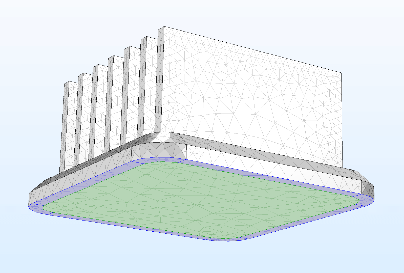Finite element discretization of the heat sink model from the earlier figure. Finite element discretization of the rut sink model from the earlier figure.

In one case the system is discretized and the boundary weather condition are imposed, a arrangement of equations is obtained according to the post-obit expression:

^(eighteen)

where T is the vector of unknowns, T _h = {T_ane, .., T_i, …, T_n }, and A is an nxn matrix containing the coefficients of T_i in each equation j within its components A_ji . The right-hand side is a vector of the dimension 1 to due north. A is the system matrix, oftentimes referred to every bit the (eliminated) stiffness matrix, harkening back to the finite element method'southward offset application likewise equally its use in structural mechanics.

If the source function is nonlinear with respect to temperature or if the estrus transfer coefficient depends on temperature, then the equation arrangement is also nonlinear and the vector b becomes a nonlinear role of the unknown coefficients T_i .

One of the benefits of the finite element method is its ability to select test and footing functions. It is possible to select examination and basis functions that are supported over a very pocket-sized geometrical region. This implies that the integrals in Eq. (17) are nada everywhere, except in very limited regions where the functions ψ_j and ψ_i overlap, as all of the above integrals include products of the functions or gradients of the functions i and j. The support of the test and ground functions is difficult to describe in 3D, simply the 2nd analogy tin can exist visualized.

Presume that there is a second geometrical domain and that linear functions of 10 and y are selected, each with a value of one at a point i, but nothing at other points k. The side by side stride is to discretize the 2d domain using triangles and depict how two basis functions (test or shape functions) could appear for two neighboring nodes i and j in a triangular mesh.

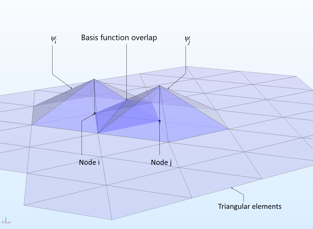Tent-shaped linear ground functions that accept a value of 1 at the respective node and zero on all other nodes. Two base functions that share an element accept a footing function overlap. Tent-shaped linear basis functions that have a value of 1 at the corresponding node and zero on all other nodes. Ii base of operations functions that share an chemical element have a footing office overlap.

Two neighboring footing functions share 2 triangular elements. As such, there is some overlap between the ii footing functions, every bit shown above. Further, note that if i = j, then there is a complete overlap between the functions. These contributions form the coefficients for the unknown vector T that correspond to the diagonal components of the system matrix A_jj .

Say the 2 basis functions are now a little further apart. These functions do not share elements but they take one element vertex in common. As the figure beneath indicates, they do not overlap.

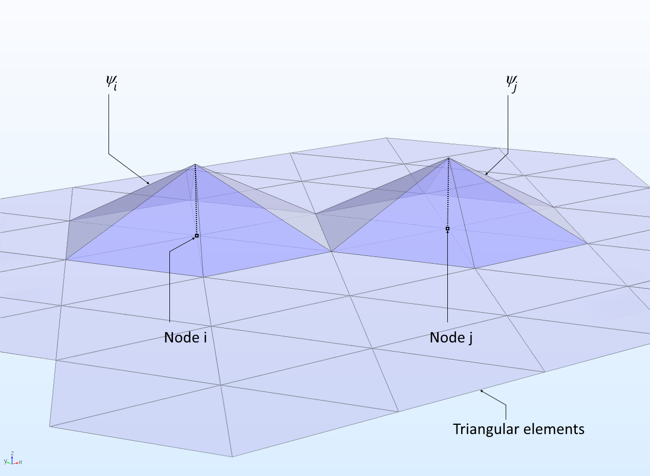Two basis functions that share one element vertex but exercise non overlap in a 2d domain. Two ground functions that share one element vertex but practice not overlap in a 2D domain.

When the basis functions overlap, the integrals in Eq. (17) have a nonzero value and the contributions to the arrangement matrix are nonzero. When there is no overlap, the integrals are zilch and the contribution to the organisation matrix is therefore nothing too.

This ways that each equation in the arrangement of equations for (17) for the nodes 1 to n only gets a few nonzero terms from neighboring nodes that share the same element. The system matrix A in Eq. (xviii) becomes sparse, with nonzero terms only for the matrix components that stand for to overlapping ij:s. The solution of the system of algebraic equations gives an approximation of the solution to the PDE. The denser the mesh, the closer the approximate solution gets to the actual solution.

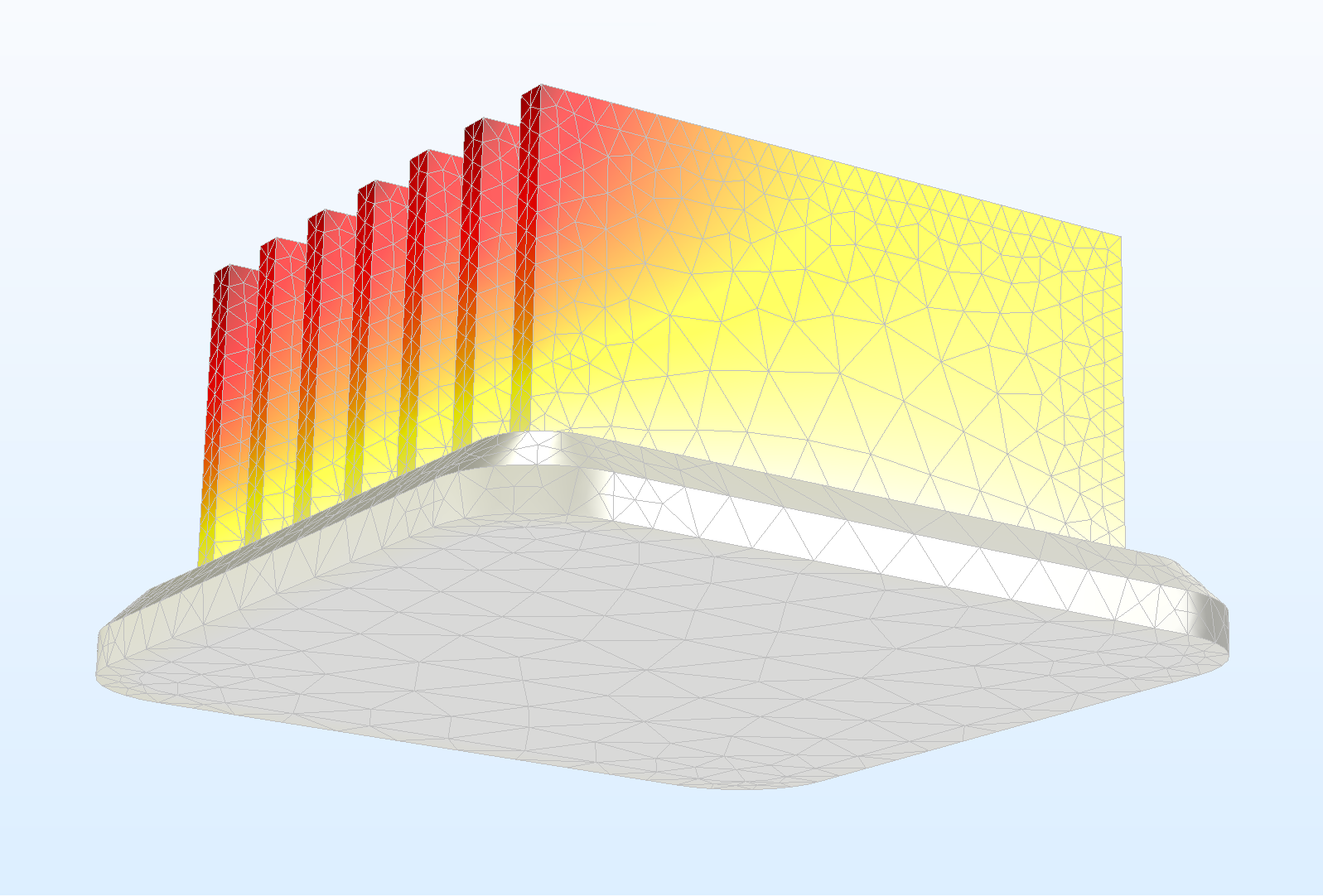The finite chemical element approximation of the temperature field in the heat sink. The finite element approximation of the temperature field in the heat sink.

Time-Dependent Issues

The thermal energy balance in the heat sink tin can be further defined for time-dependent cases. The discretized weak formulation for every test function ψ_j , using the Galerkin method, tin can so be written as:

⁽¹⁹⁾

Here, the coefficients T_i are time-dependent functions while the basis and exam functions depend but on spatial coordinates. Further, the time derivative is not discretized in the time domain.

I arroyo would be to apply FEM for the time domain equally well, but this can be rather computationally expensive. Alternatively, an contained discretization of the time domain is oftentimes applied using the method of lines. For example, information technology is possible to utilize the finite difference method. In its simplest course, this can exist expressed with the following divergence approximation:

^(twenty)

Ii potential finite difference approximations of the problem in Eq. (19) are given. The first formulation is when the unknown coefficients T_i,t are expressed in terms of t + Δt:

⁽²¹⁾

If the problem is linear, a linear system of equations needs to be solved for each time step. If the problem is nonlinear, a corresponding nonlinear organization of equations must be solved in each fourth dimension pace. The fourth dimension-marching scheme is referred to as an implicit method, as the solution at t + Δt is implicitly given by Eq. (21).

The 2d formulation is in terms of the solution at t:

⁽²²⁾

This formulation implies that once the solution (T_i,t ) is known at a given time, and so Eq. (22) explicitly gives the solution at t + Δt (T_{i, t+Δt} ). In other words, for an explicit fourth dimension-marching scheme, in that location is no demand to solve an equation system at each time pace. The drawback with explicit time-marching schemes is that they come with a stability time-stepping brake. For heat bug, like the case highlighted here, an explicit method requires very small fourth dimension steps. The implicit schemes allow for larger time steps, cutting the costs for equations like (22) that have to be solved in each time step.

In practice, modern time-stepping algorithms automatically switch between explicit and implicit steps depending on the problem. Further, the difference equation in Eq. (xx) is replaced with a polynomial expression that may vary in order and stride length depending on the problem and the development of the solution with time. A modern time-marching scheme has automatic control of the polynomial order and the stride length for the fourth dimension development of the numerical solution.

When it comes to the well-nigh mutual methods that are used, here are a few examples:

• Backwards differentiation formula (BDF) method
• Generalized alpha method
• Dissimilar Runge-Kutta methods

Different Elements

As mentioned above, the Galerkin method utilizes the same ready of functions for the basis functions and the exam functions. Yet, even for this method, there are many ways (infinitely many, in theory) of defining the basis functions (i.e., the elements in a Galerkin finite element formulation). Allow's review some of the most mutual elements.

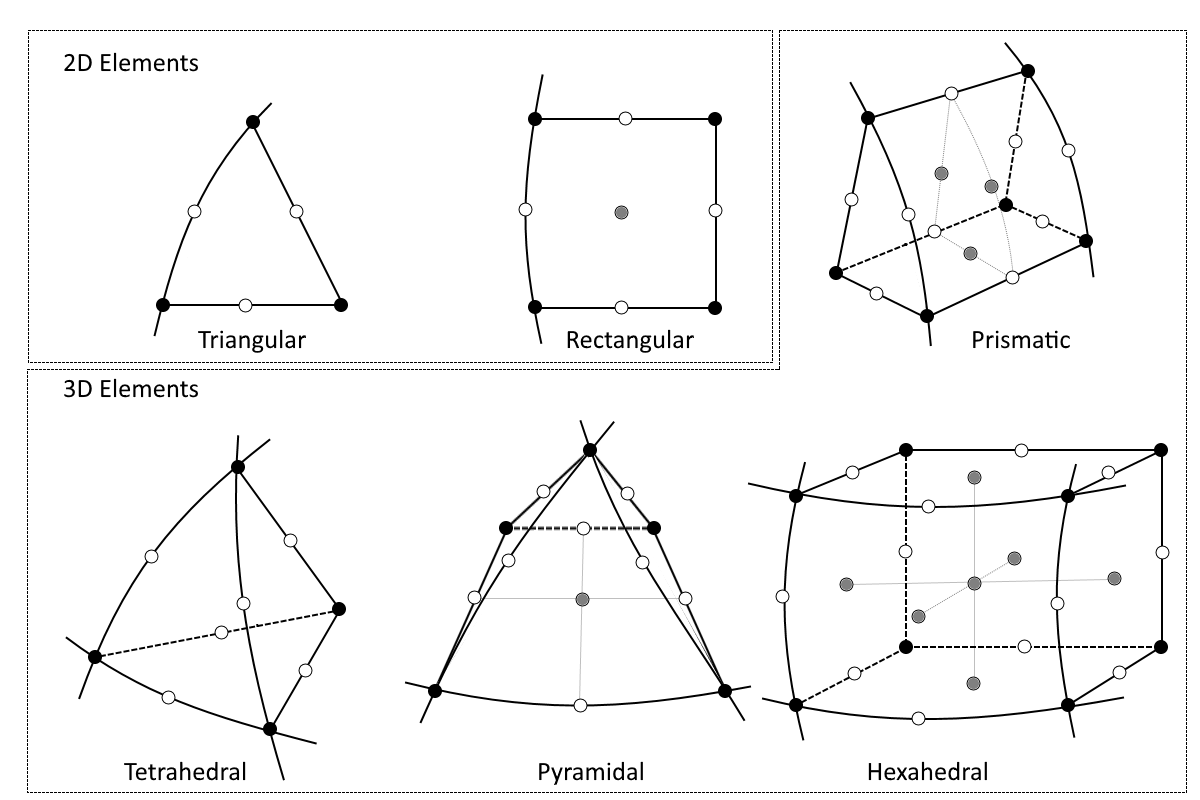
For linear functions in 2D and 3D, the nearly mutual elements are illustrated in the figure below. The linear basis functions, every bit divers in a triangular mesh that forms triangular linear elements, are depicted in this effigy and this figure above. The ground functions are expressed equally functions of the positions of the nodes (x and y in 2d and 10, y, and z in 3D).

In second, rectangular elements are often practical to structural mechanics analyses. They can also exist used for boundary layer meshing in CFD and heat transfer modeling. Their 3D analogy is known equally the hexahedral elements, and they are usually applied to structural mechanics and boundary layer meshing besides. In the transition from hexahedral boundary layer elements to tetrahedral elements, pyramidal elements are normally placed on elevation of the purlieus layer elements.

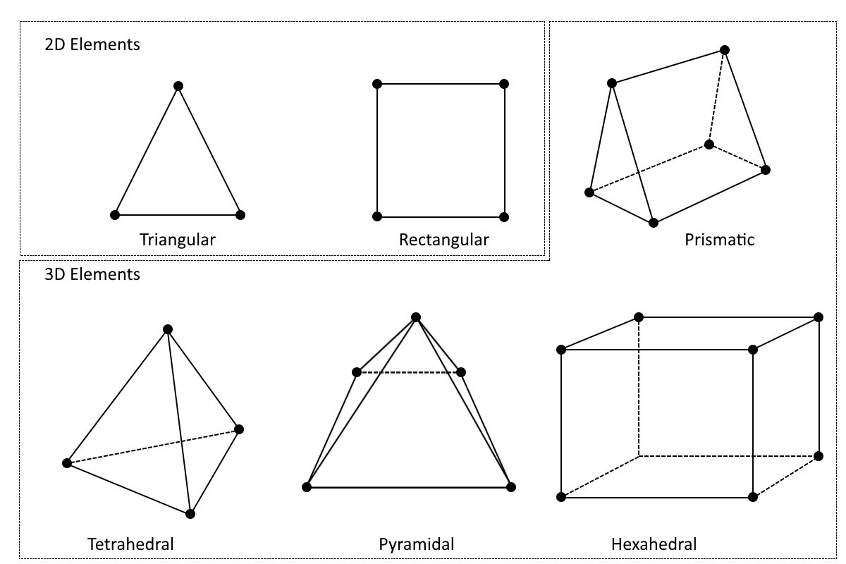Node placement and geometry for 2D and 3D linear elements. Node placement and geometry for 2nd and 3D linear elements.

The corresponding second-gild elements (quadratic elements) are shown in the figure below. Here, the edges and surfaces facing a domain boundary are frequently curved, while the edges and surfaces facing the internal portion of the domain are lines or flat surfaces. Note, yet, that at that place is as well the option to define all edges and surfaces equally curved. Lagrangian and serendipity elements are the nearly common element types in 2d and 3D. The Lagrangian elements apply all of the nodes below (black, white, and gray), while the serendipity elements omit the gray nodes.

2d-order elements. If the gray nodes are removed, we get the corresponding serendipity elements. The black, white, and grey nodes are all present in the Lagrangian elements. Second-order elements. If the gray nodes are removed, we become the corresponding serendipity elements. The black, white, and grayness nodes are all present in the Lagrangian elements.

Beautiful plots of 2d second-order (quadratic) Lagrangian elements can be found in the weblog postal service "Keeping Track of Chemical element Society in Multiphysics Models". It is difficult to depict the basis of the quadratic ground functions in 3D inside the elements above, simply color fields can be used to plot function values on the chemical element surfaces.

When discussing FEM, an important chemical element to consider is the mistake guess. This is because when an estimated error tolerance is reached, convergence occurs. Note that the discussion here is more general in nature rather than specific to FEM.

The finite element method gives an guess solution to the mathematical model equations. The difference betwixt the solution to the numerical equations and the exact solution to the mathematical model equations is the error: due east = u - u_h .

In many cases, the error can be estimated before the numerical equations are solved (i.e., an a priori error estimate). A priori estimates are often used solely to predict the convergence order of the applied finite element method. For instance, if the problem is well posed and the numerical method converges, the norm of the error decreases with the typical element size h according to O(h^α ), where α denotes the gild of convergence. This simply indicates how fast the norm of the error is expected to decrease every bit the mesh is made denser.

An a priori gauge can merely be found for simple problems. Furthermore, the estimates ofttimes contain different unknown constants, making quantitative predictions impossible. An a posteriori judge uses the estimate solution, in combination with other approximations to related issues, in social club to approximate the norm of the error.

Method of Manufactured Solutions

A very simple, only general, method for estimating the error for a numerical method and PDE problem is to modify the problem slightly, as seen in this blog post, so that a predefined belittling expression is the true solution to the modified problem. The reward here is that at that place are no assumptions made regarding the numerical method or the underlying mathematical problem. Additionally, since the solution is known, the error can easily exist evaluated. By selecting the belittling expression with care, unlike aspects of the method and problem tin can exist studied.

Allow's take a look at an example to clarify this. Assume that there is a numerical method that solves Poisson's equation on a unit square (Ω) with homogeneous boundary conditions

⁽²³⁾

⁽²⁴⁾

This method can exist used to solve a modified problem

⁽²⁵⁾

⁽²⁶⁾

where

⁽²⁷⁾

Here,

is an belittling expression that can be selected freely. If also

⁽²⁸⁾

then is the exact solution to the modified problem and the error can exist direct evaluated:

⁽²⁹⁾

The error and its norm tin can at present be computed for unlike choices of discretization and different choices of . The error to the modified trouble can be used to guess the mistake for the unmodified trouble if the graphic symbol of the solution to the modified problem resembles the solution to the unmodified trouble. In exercise, it may be difficult to know if this is the case – a drawback of the technique. The strength of the approach lies in its simplicity and generality. Information technology can be used for nonlinear and fourth dimension-dependent problems, and it can be used for any numerical method.

Goal-Oriented Estimates

If a office, or functional, is selected every bit an of import quantity to estimate from the approximate solution, and so analytical methods can be used to derive sharp mistake estimates, or bounds, for the computational error made for this quantity. Such estimates rely on a posteriori evaluation of a PDE residual and computation of the approximation to a so-called dual problem. The dual problem is directly related to (and defined by) the selected office.

The drawback of this method is that it hinges on the accurate ciphering of the dual problem and merely gives an estimate of the fault for the selected function, non for other quantities. Its strength lies in the fact that information technology is rather generally applicative and the error is computable with reasonable efforts.

Mesh Convergence

Mesh convergence is a elementary method that compares approximate solutions obtained for unlike meshes. Ideally, a very fine mesh approximation solution tin can exist taken as an approximation to the actual solution. The error for approximation on the coarser meshes can then be directly evaluated every bit

⁽³⁰⁾

In exercise, calculating an approximation for a very much effectively mesh than those of interest tin can be difficult. Therefore, information technology is customary to use the finest mesh approximation for this purpose. It is also possible to guess the convergence from the change in the solution for each mesh refinement. The change in the solution should go smaller for each mesh refinement if the approximate solution is in a converging expanse, and then that it moves closer and closer to the existent solution.

The figure below shows a structural mechanics criterion model for an elliptic membrane where just ane 4th of the membrane is treated cheers to symmetry. The load is applied on the outer edge of the geometry while symmetry is causeless at the boundaries along the 10- and y-axis.

Benchmark model of an elliptic membrane. The load is applied at the outer edge while symmetry is assumed at the edges positioned forth the ten- and y-axis (roller support).

Criterion model of an elliptic membrane. The load is applied at the outer edge while symmetry is causeless at the edges positioned along the x- and y-centrality (roller support).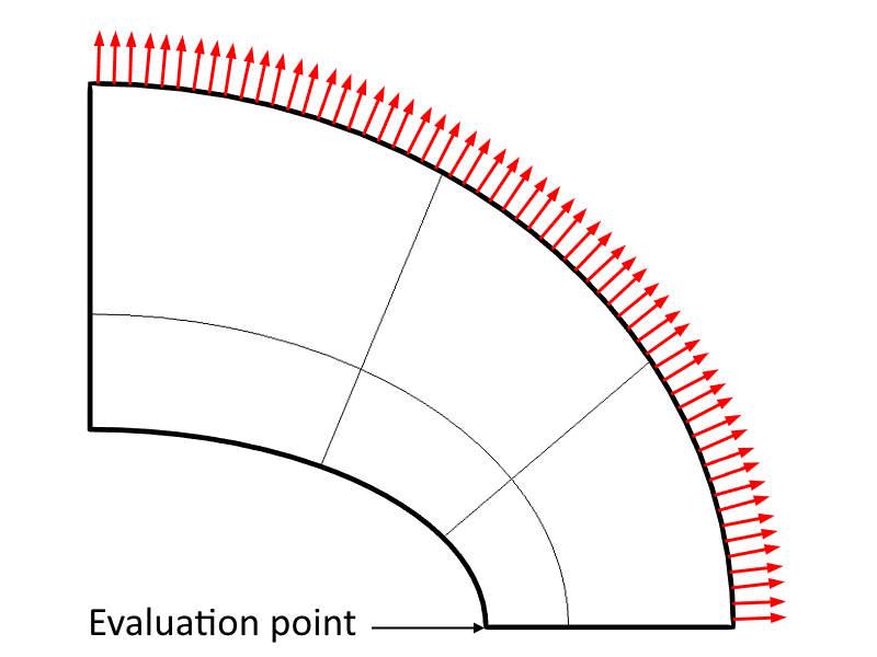

The numerical model equations are solved for different mesh types and element sizes. For example, the effigy below depicts the rectangular Lagrange elements used for the quadratic basis functions according this previous figure.

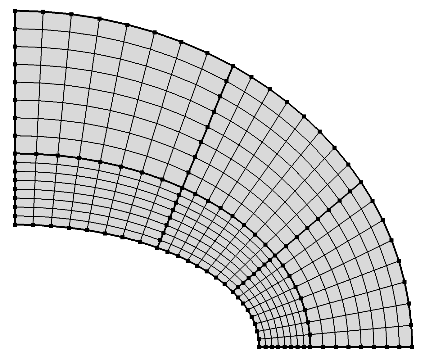Rectangular elements used for the quadratic base of operations functions. Rectangular elements used for the quadratic base functions.

The stresses and strains are evaluated in the point according to this before effigy. The relative values obtained for σ_x at this bespeak are shown in the nautical chart beneath. This value should be zero and any departure from zero is therefore an error. To get a relative error, the computed σ₁₀ is divided past the computed σ_y in order to get the right order of magnitude for a relative mistake judge.

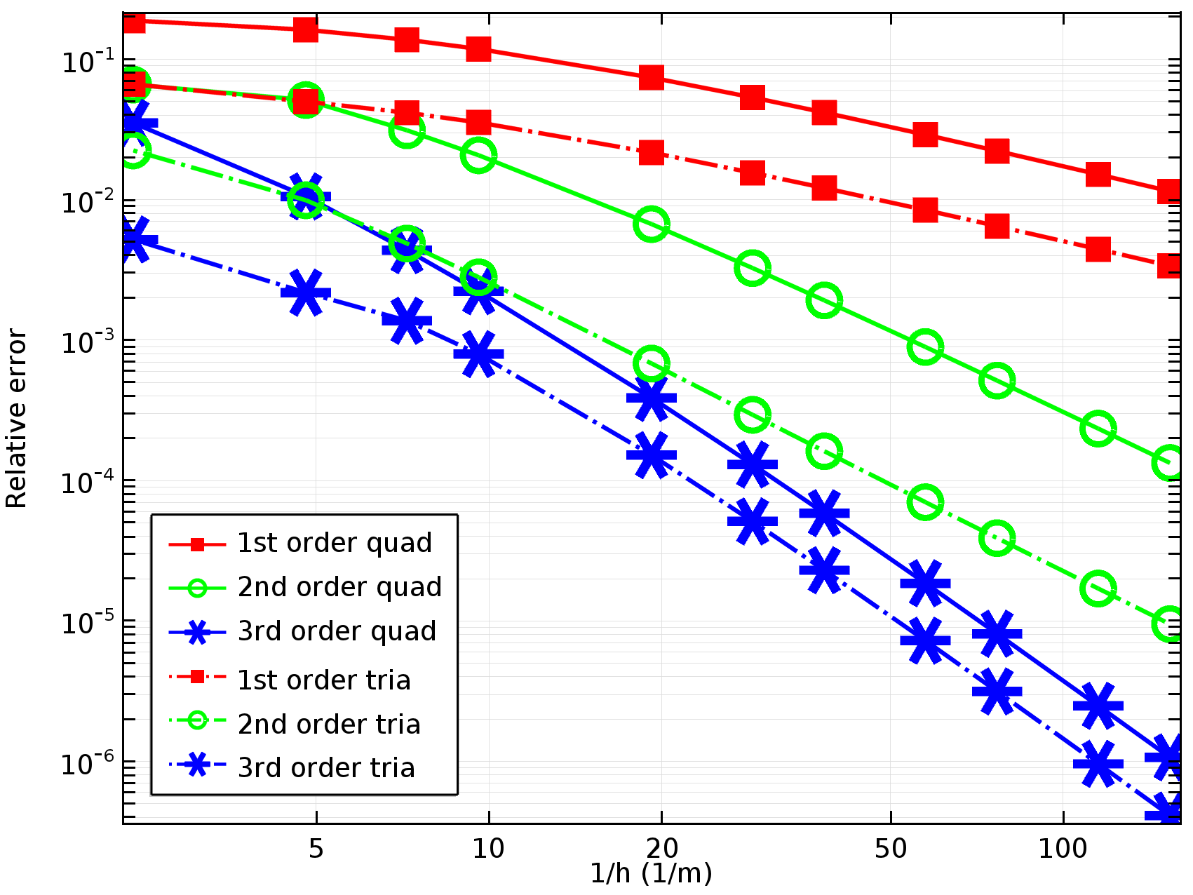Relative error in σ_x at the evaluation betoken in the previous figure for different elements and element sizes (element size = h). Quad refers to rectangular elements, which can be linear or with quadratic ground functions. Relative error in σ_x at the evaluation indicate in the previous figure for different elements and element sizes (element size = h). Quad refers to rectangular elements, which can be linear or with quadratic ground functions.

The higher up plot shows that the relative error decreases with decreasing element size (h) for all elements. In this case, the convergence bend becomes steeper as the gild of the basis functions (elements order) becomes higher. Annotation, however, that the number of unknowns in the numerical model increases with the chemical element order for a given element size. This means that when we increment the guild of the elements, we pay the price for higher accurateness in the form of increased computational time. An alternative to using higher-lodge elements is therefore to implement a finer mesh for the lower-order elements.

Mesh Adaptation

After computing a solution to the numerical equations, u_h , a posteriori local error estimates tin be used to create a denser mesh where the fault is large. A second guess solution may and then exist computed using the refined mesh.

The figure below depicts the temperature field around a heated cylinder subject to fluid period at steady state. The stationary problem is solved twice: once with the basic mesh and once with a refined mesh controlled by the error estimation that is computed from the basic mesh. The refined mesh provides higher accuracy in temperature and heat flux, which may exist required in this specific example.

Temperature field around a heated cylinder that is subjected to a flow computed without mesh refinement (summit) and with mesh refinement (lesser). Temperature field effectually a heated cylinder that is subjected to a flow computed without mesh refinement (peak) and with mesh refinement (lesser).

For convective time-dependent problems, in that location is likewise the pick to convect the refinement of the mesh via the solution in a previous time step. For instance, in the figure below, the phase field is used to compute the interface between an ink droplet and air in an inkjet. The interface is given by the isosurface of the phase field part, where its value is equal to 0.5. At this interface, the phase field function goes from 1 to 0 very rapidly. Nosotros tin can use the error gauge to automatically refine the mesh around these steep gradients of the phase field function, and the catamenia field can exist used to convect the mesh refinement to utilise a finer mesh just in front of the phase field isosurface.

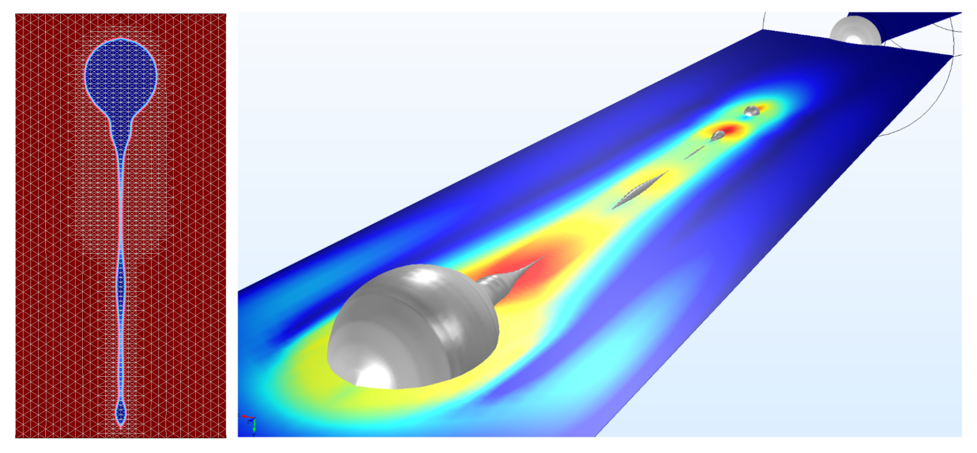The mesh refinement follows the train of droplets from an inkjet in a time-dependent, ii-stage flow problem. The mesh refinement follows the railroad train of droplets from an inkjet in a fourth dimension-dependent, two-phase flow trouble.

Additional Finite Element Formulations

In the examples above, nosotros have formulated the discretization of the model equations using the same ready of functions for the basis and test functions. One finite element formulation where the examination functions are different from the footing functions is called a Petrov-Galerkin method. This method is common, for example, in the solution of convection-diffusion problems to implement stabilization only to the streamline direction. Information technology is also referred to every bit the streamline upwind/Petrov-Galerkin (SUPG) method.

In the solution of coupled systems of equations, different basis functions may be used for different dependent variables. A typical instance is the solution of the Navier-Stokes equations, where the force per unit area is often more smoothen and piece of cake to approximate than the velocity. Methods where the footing (and test) functions for different dependent variables in a coupled system belong to different part spaces are called mixed finite element methods.

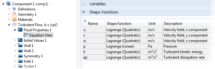Settings for a mixed chemical element method for fluid flow in COMSOL Multiphysics software, where quadratic shape functions (footing functions) are used for velocity and linear shape functions are used for pressure. Settings for a mixed chemical element method for fluid menstruum in COMSOL Multiphysics software, where quadratic shape functions (basis functions) are used for velocity and linear shape functions are used for pressure.

Published: March 15, 2016
Last modified: Feb 21, 2017

joyalsarronever78.blogspot.com

Source: https://www.comsol.com/multiphysics/finite-element-method

Share this post